Quickstart Tutorial
Description
rodeo is a fast Python library that uses probabilistic numerics to solve ordinary differential equations (ODEs). That is, most ODE solvers (such as Euler’s method) produce a deterministic approximation to the ODE on a grid of step size \(\Delta t\). As \(\Delta t\) goes to zero, the approximation converges to the true ODE solution. Probabilistic solvers also output a solution on a grid of size \(\Delta t\); however, the solution is random. Still, as \(\Delta t\) goes to zero, the probabilistic numerical approximation converges to the true solution.
For the basic task of solving ODEs, rodeo provides a probabilistic solver, rodeo, for univariate process \(x(t)\) of the form
where \(\xx(t) = \big(x^{(0)}(t), x^{(1)}(t), ..., x^{(q-1)}(t)\big)\) consists of \(x(t)\) and its first \(q-1\) derivatives, \(\WW\) is a coefficient matrix, and \(f(\xx(t), t)\) is typically a nonlinear function.
rodeo begins by putting a Gaussian process prior on the ODE solution, and updating it sequentially as the solver steps through the grid.
import jax
import jax.numpy as jnp
import numpy as np
import matplotlib.pyplot as plt
from scipy.integrate import odeint

import rodeo
from rodeo.prior import ibm_init
from rodeo import solve_mv, solve_sim
from rodeo.utils import first_order_pad
from jax import config
config.update("jax_enable_x64", True)
Walkthrough
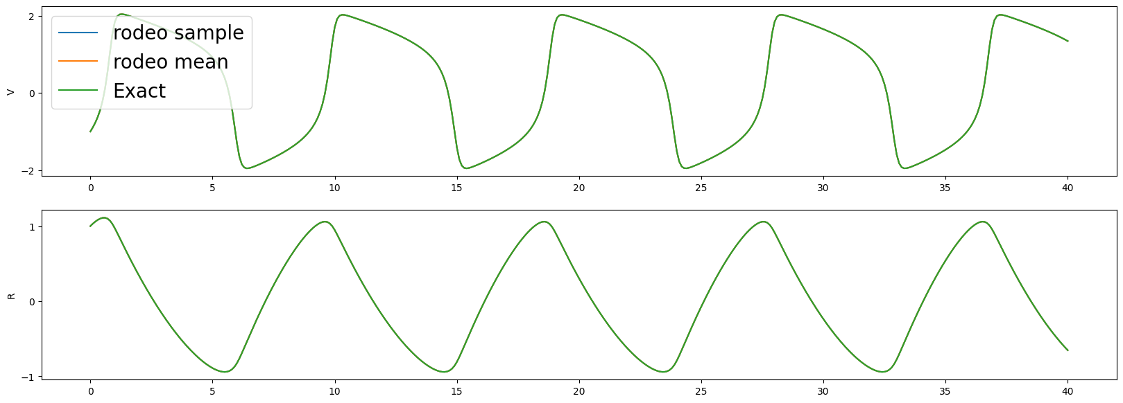
To illustrate the set-up, let’s consider the following ODE example (FitzHugh-Nagumo model) where \(p=2\) for both variables:
where the solution \(X(t)\) is sought on the interval \(t \in [0, 40]\) and \(\theta = (a,b,c) = (.2,.2,3)\).
To approximate the solution with the probabilistic solver, we use a simple Gaussian process prior proposed by Schober et al (2019); namely, that \(V(t)\) and \(R(t)\) are independent \(q-1\) times integrated Brownian motion, such that
for \(x=V, R\). The result is a \(q\)-dimensional continuous Gaussian Markov process \(\boldsymbol{x(t)} = \big(x^{(0)}(t), x^{(1)}(t), \ldots, x^{(q-1)}(t)\big)\) for each variable \(x=V, R\). The IBM model specifies that each of these is continuous, but \(x^{(q)}(t)\) is not. Therefore, we need to pick \(q \geq p\). It’s usually a good idea to have \(q\) a bit larger than \(p\), especially when we think that the true solution \(X(t)\) is smooth. However, increasing \(q\) also increases the computational burden, and doesn’t necessarily have to be large for the solver to work. For this example, we will use \(q=3\). To initialize, we simply set \(\boldsymbol{X(0)} = (V^{(0)}(0), V^{(1)}(0), 0, R^{(0)}(0), R^{(1)}(0), 0)\) where we padded the initial value with zeros for the higher derivative. The Python code to implement all this is as follows.
def fitz_fun(X_t, t, **params):
    "FitzHugh-Nagumo ODE."
    a, b, c = params["theta"]
    V, R = X_t[:,0]
    return jnp.array([[c*(V - V*V*V/3 + R)],
                    [-1/c*(V - a + b*R)]])


# problem setup and intialization
n_vars = 2  # number of variables
n_deriv = 3 # q

# it is assumed that the solution is sought on the interval [tmin, tmax].
n_steps = 400
t_min = 0.
t_max = 40.
theta = jnp.array([0.2, 0.2, 3])

# The rest of the parameters can be tuned according to ODE
# For this problem, we will use
sigma = .01
sigma = jnp.array([sigma]*n_vars)

# Initial W for jax block
W, fitz_init_pad = first_order_pad(fitz_fun, n_vars, n_deriv)

# Initial x0 for jax block
theta = jnp.array([0.2, 0.2, 3])  # ODE parameters
x0 = jnp.array([-1.0, 1.0])  # initial value for the ODE-IVP
X0 = fitz_init_pad(x0, 0, theta=theta)  # initial value in rodeo format

# Get parameters needed to run the solver
dt = (t_max-t_min)/n_steps
prior_pars = ibm_init(dt, n_deriv, sigma)
One of the key steps in the probabilisitc solver is the interrogation step. We offer several choices for this task: interrogate_schober by Schober et al (2019), interrogate_chkrebtii by Chkrebtii et al (2016), interrogate_rodeo which is a mix of the two, and interrogate_kramer by Kramer et al (2021).
interrogate_schoberis the simplest and fastest.interrogate_chkrebtiiis a Monte Carlo method that returns a non-deterministic output which does not assume zero variance like Schober et al (2019) and Tronarp et al (2018).interrogate_krameris an extension tointerrogate_schoberwhere a first order Taylor approximation is used which has shown to have better numerical stability.
We recommend interrogate_kramer for general problems.
rodeo offers two output functions: solve_sim and solve_mv. The former returns a sample from the solution posterior, \(\xx_{0:N}\) and the latter returns the posterior mean, \(\mmu_{0:N}\) and variance \(\SSi_{0:N|N}\). The next step is optional but significantly speeds up the solver if the ODE is solved many times. This uses jax.jit to jit-compile the solver. Note that there are 3 static arguments which are either function or integer inputs.
# Jit solver
key = jax.random.PRNGKey(0)
sim_jit = jax.jit(solve_sim, static_argnums=(1, 6, 7))
mv_jit = jax.jit(solve_mv, static_argnums=(1, 6, 7))

xt = sim_jit(key=key, ode_fun=fitz_fun,
             ode_weight=W, ode_init=X0, theta=theta,
             t_min=t_min, t_max=t_max, n_steps=n_steps,
             interrogate=rodeo.interrogate.interrogate_kramer,
             prior_pars=prior_pars)
mut, _ = mv_jit(key=key, ode_fun=fitz_fun,
             ode_weight=W, ode_init=X0, theta=theta,
             t_min=t_min, t_max=t_max, n_steps=n_steps,
             interrogate=rodeo.interrogate.interrogate_kramer,
             prior_pars=prior_pars)
To compare the rodeo solution, we use the deterministic solution provided by odeint.
def ode_fun(X_t, t, theta):
    a, b, c = theta
    V, R = X_t
    return np.array([c*(V - V*V*V/3 + R), -1/c*(V - a + b*R)])

# Initial x0 for odeint
ode0 = np.array([-1., 1.])

# Get odeint solution for Fitz-Hugh
tseq = np.linspace(t_min, t_max, n_steps+1)
exact = odeint(ode_fun, ode0, tseq, args=(theta,))

# Graph the results
fig, axs = plt.subplots(2, 1, figsize=(20, 7))
ylabel = ['V', 'R']
plt.rcParams.update({'font.size': 20})
for i in range(2):
    axs[i].plot(tseq, xt[:, i, 0], label="rodeo sample")
    axs[i].plot(tseq, mut[:, i, 0], label="rodeo mean")
    axs[i].set_ylabel(ylabel[i])
    axs[i].plot(tseq, exact[:, i], label='Exact')
axs[0].legend(loc='upper left')
<matplotlib.legend.Legend at 0x74e678295880>