Parameter Inference

In this notebook, we demonstrate the steps to conduct parameter inference using various likelihood approximation methods in rodeo.

# --- 0. Import libraries and modules ------------------------------------


import jax
import jax.numpy as jnp
import jaxopt
import blackjax
from functools import partial
import rodeo
from rodeo.prior import ibm_init
from rodeo.solve import solve_mv, solve_sim
from rodeo.interrogate import interrogate_chkrebtii, interrogate_kramer
from rodeo.inference import basic, fenrir, pseudo_marginal
from rodeo.utils import first_order_pad

import matplotlib.pyplot as plt
import seaborn as sns
from jax import config
config.update("jax_enable_x64", True)

Walkthrough

We will use the FitzHugh-Nagumo model as the example here which is a two-state ODE on \(\xx(t) = (V(t), R(t))\),

\[\begin{align*} \frac{dV(t)}{dt} &= c(V(t) - \frac{V(t)^3}{3} + R(t)), \\ \frac{dR(t)}{dt} &= -\frac{(V(t) - a + bR(t))}{c}. \\ \end{align*}\]

The model parameters are \(\tth = (a,b,c,V(0),R(0))\), with \(a,b,c > 0\) which are to be learned from the measurement model

\[\begin{align*} \YY_i \sim \N(\xx(t_i), \phi^2 \Id_{2 \times 2}) \end{align*}\]

where \(t_i = i\) and \(i=0,1,\ldots 40\) and \(\phi^2 = .04\). We will first simulate some noisy data using an highly accurate ODE solver (odeint).

# --- 1. Define the ODE-IVP ----------------------------------------------


def fitz_fun(X, t, **params):
    "FitzHugh-Nagumo ODE in rodeo format."
    a, b, c = params["theta"]
    V, R = X[:, 0]
    return jnp.array(
        [[c * (V - V * V * V / 3 + R)],
         [-1 / c * (V - a + b * R)]]
    )


n_vars = 2
n_deriv = 3

x0 = jnp.array([-1., 1.])  # initial value for the ODE-IVP
theta = jnp.array([.2, .2, 3])  # ODE parameters

# helper function for standard first-order problems where W is fixed, it returns
# W: LHS matrix of ODE
# fitz_init_pad: Function to help initialize FN model with
# Args: x0, t, **params
# Returns: Function that takes the initial values of each variable
#          and puts them in rodeo format.
W, fitz_init_pad = first_order_pad(fitz_fun, n_vars, n_deriv)
X0 = fitz_init_pad(x0, 0, theta=theta)  # initial value in rodeo form

# Time interval on which a solution is sought.
t_min = 0.
t_max = 40.

# --- Define the prior process -------------------------------------------

# IBM process scale factor
sigma = jnp.array([.1] * n_vars)


# --- data simulation ------------------------------------------------------


dt_obs = 1.  # interobservation time
n_steps_obs = int((t_max - t_min) / dt_obs)
# observation times
obs_times = jnp.linspace(t_min, t_max,
                         num=n_steps_obs + 1)

# number of simulation steps per observation
n_res = 20
n_steps = n_steps_obs * n_res
# simulation times
sim_times = jnp.linspace(t_min, t_max,
                         num=n_steps + 1)

# prior parameters
dt_sim = (t_max - t_min) / n_steps  # grid size for simulation
prior_pars = rodeo.prior.ibm_init(
    dt=dt_sim,
    n_deriv=n_deriv,
    sigma=sigma
)

# Produce a Pseudo-RNG key
key = jax.random.PRNGKey(100)


# calculate ODE via deterministic output
key, subkey = jax.random.split(key)
Xt, _ = rodeo.solve_mv(
    key=subkey,
    # define ode
    ode_fun=fitz_fun,
    ode_weight=W,
    ode_init=X0,
    t_min=t_min,
    t_max=t_max,
    theta=theta,  # ODE parameters added here
    # solver parameters
    n_steps=n_steps,
    interrogate=rodeo.interrogate.interrogate_kramer,
    prior_pars=prior_pars
)

# generate observations
noise_sd = jnp.sqrt(0.005)  # Standard deviation in noise model
key, subkey = jax.random.split(key)
eps = jax.random.normal(
    key=subkey,
    shape=(obs_times.size, 2)
)
# 0th order derivatives at observed timepoints
obs_ind = jnp.searchsorted(sim_times, obs_times)
x = Xt[obs_ind, :, 0]
Y = x + noise_sd * eps

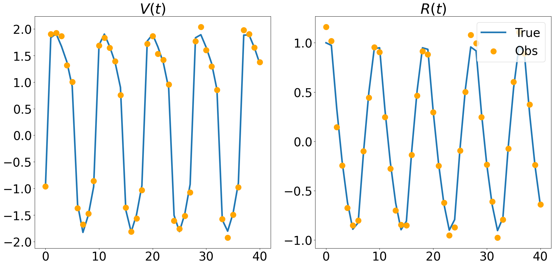
Observations are available at \(t=0,1,\ldots, 40\). However, the ODE solver requires a higher resolution than \(\Delta t = 1\) to give a good approximation. Here we use n_res=20 which means \(\Delta t = 1/20\).

# plot one graph
plt.rcParams.update({'font.size': 30})
fig1, axs = plt.subplots(1, 2, figsize=(20, 10))
axs[0].plot(obs_times, x[:,0], label = 'True', linewidth=4)
axs[0].scatter(obs_times, Y[:,0], label = 'Obs', color='orange', s=200, zorder=2)
axs[0].set_title("$V(t)$")
axs[1].plot(obs_times, x[:,1], label = 'True', linewidth=4)
axs[1].scatter(obs_times, Y[:,1], label = 'Obs', color='orange', s=200, zorder=2)
axs[1].set_title("$R(t)$")
axs[1].legend(loc=1)
fig1.tight_layout()

We now turn to the problem of parameter estimation. In the Bayesian context, this is achieved by postulating a prior distribution \(p(\TTh)\) on \(\TTh = (\tth, \pph)\), and then combining it with the stochastic solver’s likelihood function \(\Ell(\TTh \mid \YY_{0:M}) \propto p(\YY_{0:M} \mid \ZZ_{1:N} = \bz, \TTh)\) to obtain the posterior distribution

\[\begin{equation*} p(\TTh \mid \YY_{0:M}) \propto \pi(\TTh) \times \Ell(\TTh \mid \YY_{0:M}). \end{equation*}\]

For the Basic, Fenrir, and DALTON algorithms, the high-dimensional latent ODE variables \(\XX_{0:N}\) can be approximately integrated out to produce a closed-form likelihood approximation \(\hat \Ell(\TTh \mid \YY_{0:M})\) to form the corresponding posterior approximation \(\hat p(\TTh \mid \YY_{0:M})\). While this posterior can be readily sampled from using MCMC techniques (as we shall do momentarily) Bayesian parameter estimation can also be achieved by way of a Laplace approximation. We approximate, \(p(\TTh \mid \YY_{0:M})\) is approximated by a multivariate normal distribution,

\[\begin{equation*} \TTh \mid \YY_{0:M} \approx \N(\hat \TTh, \hat \VV), \end{equation*}\]

where

\[\begin{align*} \hat \TTh & = \argmax_{\TTh} \log \hat p(\TTh \mid \YY_{0:M}), & \hat \VV & = -\left[\frac{\partial^2}{\partial \TTh \partial \TTh'} \log \hat p(\hat \TTh \mid \YY_{0:M})\right]^{-1}. \end{align*}\]

# --- parameter inference: basic + laplace -------------------------------

def fitz_logprior(upars):
    "Logprior on unconstrained model parameters."
    n_theta = 5  # number of ODE + IV parameters
    lpi = jax.scipy.stats.norm.logpdf(
        x=upars[:n_theta],
        loc=0.,
        scale=10.
    )
    return jnp.sum(lpi)


def fitz_loglik(obs_data, ode_data, **params):
    """
    Loglikelihood for measurement model.

    Args:
        obs_data (ndarray(n_obs, n_vars)): Observations data.
        ode_data (ndarray(n_obs, n_vars, n_deriv)): ODE solution.
    """
    ll = jax.scipy.stats.norm.logpdf(
        x=obs_data,
        loc=ode_data[:, :, 0],
        scale=noise_sd
    )
    return jnp.sum(ll)


def fitz_constrain_pars(upars, dt):
    """
    Convert unconstrained optimization parameters into rodeo inputs.

    Args:
        upars : Parameters vector on unconstrainted scale.
        dt : Discretization grid size.

    Returns:
        tuple with elements:
        - theta : ODE parameters.
        - X0 : Initial values in rodeo format.
        - prior_pars : Prior matrices.
    """
    theta = jnp.exp(upars[:3])
    x0 = upars[3:5]
    X0 = fitz_init_pad(x0, 0, theta=theta)
    sigma = upars[5:]
    prior_pars = rodeo.prior.ibm_init(
        dt=dt,
        n_deriv=n_deriv,
        sigma=sigma
    )
    return theta, X0, prior_pars


def fitz_laplace(key, neglogpost, n_samples, upars_init):
    """
    Sample from the Laplace approximation to the parameter posterior for the FN model.

    Args:
        key : PRNG key.
        neglogpost: Function specifying the negative log-posterior distribution
                    in terms of the unconstrained parameter vector ``upars``.
        upars_init: Initial value to the optimization algorithm over ``neglogpost()``.
        n_samples : Number of posterior samples to draw.

    Returns:
        JAX array of shape ``(n_samples, 5)`` of posterior samples from ``(theta, x0)``.
    """
    n_theta = 5  # number of ODE + IV parameters
    # find mode of neglogpost()
    solver = jaxopt.ScipyMinimize(
        fun=neglogpost,
        method="Newton-CG",
        jit=True
    )
    opt_res = solver.run(upars_init)
    upars_mean = opt_res.params
    # variance estimate
    upars_fisher = jax.jacfwd(jax.jacrev(neglogpost))(upars_mean)
    # unconstrained ode+iv parameter variance estimate
    uode_var = jax.scipy.linalg.inv(upars_fisher[:n_theta, :n_theta])
    uode_mean = upars_mean[:n_theta]
    # sample from Laplace approximation
    uode_sample = jax.random.multivariate_normal(
        key=key,
        mean=uode_mean,
        cov=uode_var,
        shape=(n_samples,)
    )
    # convert back to original scale
    ode_sample = uode_sample.at[:, :3].set(jnp.exp(uode_sample[:, :3]))
    return ode_sample

Basic Likelihood

A basic approximation to the likelihood function takes the posterior mean \(\mmu_{0:N|N}(\tth, \eet) = \E_\L[\XX_{0:N} \mid \ZZ_{1:N} = \bz, \tth, \eet]\) of the rodeo solver and simply plugs it into the measurement model, such that

\[\begin{equation*} \hat \Ell(\TTh \mid \YY_{0:M}) = \prod_{i=0}^M p(\YY_i \mid \XX_{n(i)} = \mmu_{n(i)|N}(\tth, \eet), \pph), \end{equation*}\]

where in terms of the ODE solver discretization time points \(t = t_0, \ldots, t_N\), \(N \ge M\), the mapping \(n(\cdot)\) is such that \(t_{n(i)} = t'_i\). .

def neglogpost_basic(upars):
    "Negative logposterior for basic approximation."
    # solve ODE
    theta, X0, prior_pars = fitz_constrain_pars(upars, dt_sim)
    # basic loglikelihood
    ll, Xt = rodeo.inference.basic(
        key=key,  # immaterial, since not used
        # ode specification
        ode_fun=fitz_fun,
        ode_weight=W,
        ode_init=X0,
        t_min=t_min,
        t_max=t_max,
        theta=theta,
        # solver parameters
        n_steps=n_steps,
        interrogate=rodeo.interrogate.interrogate_kramer,
        prior_pars=prior_pars,
        # observations
        obs_data=Y,
        obs_times=obs_times,
        obs_loglik=fitz_loglik
    )
    return -(ll + fitz_logprior(upars))

# optimization process
n_samples = 100000
upars_init = jnp.append(jnp.log(theta), x0)
upars_init = jnp.append(upars_init, jnp.ones(n_vars))
basic_post = fitz_laplace(key, neglogpost_basic, n_samples, upars_init)

Chkrebtii MCMC

The marginal MCMC method shares the same API as the Blackjax MCMC. The first step is to choose a proposal distribution. For this, we use a random walk (RW) kernel:

\[\begin{equation*} \TTh \mid \TTh^\curr \sim \N(\TTh^\curr, \diag(\SSi_{rw}^2)), \end{equation*}\]

where \(\diag(\SSi_{rw}^2)\) is a tuning parameter for the MCMC algorithm. While Blackjax provides a RW MCMC sampler, it does not support a Metropolis–Hastings acceptance ratio that depends on the auxiliary random variable \(\XX_{0:N}\), as required for pseudo-marginal MCMC. Therefore, we use the Blackjax API to define a pseudo-marginal MCMC sampler with an RW kernel, which we provide in the rodeo.random_walk_aux module.

There are three main steps to using the marginal MCMC method. First, a likelihood function must be defined, where the ODE solver uses the interrogation method of Chkrebtii et al (2016) to sample from the solution posterior \(\hat{p}_\L(\XX_{0:N}, \ipar_{0:N} \mid \ZZ_{1:N} = \bz, \tth, \eet)\) where \(\ipar_{0:N}\) correspond to Chkrebtii interrogations. Second, a kernel must be defined, for which we use the RW kernel. Finally, an inference loop} is used to draw MCMC samples from the parameter posterior.

interrogate_chkrebtii_partial = partial(interrogate_chkrebtii, kalman_type="standard")

def fitz_logpost_mcmc(upars, key):
    r"""
    Compute the log-posterior for Chkrebtii's marginal MCMC algorithm.
    """
    theta, X0, prior_pars = fitz_constrain_pars(upars, dt_sim)
    Xt = solve_sim(
        key=key,
        # define ode
        ode_fun=fitz_fun,
        ode_weight=W,
        ode_init=X0,
        t_min=t_min,
        t_max=t_max,
        theta=theta,
        # solver parameters
        n_steps=n_steps,
        interrogate=interrogate_chkrebtii_partial,
        prior_pars=prior_pars,
    )
    ode_data = Xt[obs_ind]
    lp = fitz_logprior(upars) + fitz_loglik(Y, ode_data)
    return lp, Xt


def fitz_marginal_mcmc(key, upars_init, n_samples):
    """
    Sample from the parameter posterior via Chkrebtii marginal MCMC.

    Args:
        key : PRNG key.
        upars_init : Initial value to the optimization algorithm.
        n_samples : Number of posterior samples to draw.
        
    Returns:
        JAX array of shape ``(n_samples, 5)`` of posterior samples from ``(theta, x0)``.
    """
    key, *subkeys = jax.random.split(key, num=3)

    # standard deviation of the random walk
    scale = jnp.array(
        [0.01, 0.1, 0.01, 0.01, 0.01, 0.01, 0.01])
    # choose the mcmc algorithm
    marginal_mcmc = pseudo_marginal.normal_random_walk(fitz_logpost_mcmc, scale)

    # initialize mcmc state
    initial_state = marginal_mcmc.init(upars_init, subkeys[0])

    # setup the kernel
    kernel = marginal_mcmc.step

    def inference_loop(key, kernel, initial_state, n_samples):
        def one_step(state, rng_key):
            state, _ = kernel(rng_key, state)
            return state, state

        keys = jax.random.split(key, n_samples)
        _, states = jax.lax.scan(one_step, initial_state, keys)
        return states

    uode_sample = inference_loop(
        subkeys[1], kernel, initial_state, n_samples).position[:, :5]
    # convert back to original scale
    ode_sample = uode_sample.at[:, :3].set(jnp.exp(uode_sample[:, :3]))
    return ode_sample

# optimization process
n_samples = 10000
upars_init = jnp.append(jnp.log(theta), x0)
upars_init = jnp.append(upars_init, .1*jnp.ones(n_vars))
mcmc_post = fitz_marginal_mcmc(key, upars_init,  n_samples)

Fenrir

The Fenrir method Tronarp et al (2022) is applicable to Gaussian measurement models of the form

\[\begin{equation*} \YY_i \ind \N(\DD_i^{(\pph)} \XX_{n(i)}, \OOm_i^{(\pph)}). \end{equation*}\]

Fenrir begins by estimating \(p_\L(\XX_{0:N} \mid \ZZ_{1:N} = \bz, \tth, \eet)\). This results in a Gaussian non-homogeneous Markov model going backwards in time,

\[\begin{align*} \XX_N & \sim \N(\bb_N, \CC_N) \\ \XX_n \mid \XX_{n+1} & \sim \N(\AA_n \XX_n + \bb_n, \CC_n), \\ \end{align*}\]

where the coefficients \(\AA_{0:N-1}\), \(\bb_{0:N}\), and \(\CC_{0:N}\) can be derived using the Kalman filtering and smoothing recursions. In combination with the Gaussian measurement model, the integral in the likelihood function can be computed analytically.

# gaussian measurement model specification in blocked form
n_meas = 1  # number of measurements per variable in obs_data_i
obs_data = jnp.expand_dims(Y, axis=-1)
obs_weight = jnp.zeros((len(obs_data), n_vars, n_meas, n_deriv))
obs_weight = obs_weight.at[:].set(jnp.array([[[1., 0., 0.]], [[1., 0., 0.]]]))
obs_var = jnp.zeros((len(obs_data), n_vars, n_meas, n_meas))
obs_var = obs_var.at[:].set(noise_sd**2 * jnp.array([[[1.]], [[1.]]]))

The way to construct a likelihood estimation is very similar to the basic method. The one difference is that fenrir asks for obs_weight and obs_var instead of obs_loglik since it assumes observations are multivariate normal.

def neglogpost_fenrir(upars):
    "Negative logposterior for basic approximation."
    theta, X0, prior_pars = fitz_constrain_pars(upars, dt_sim)
    # fenrir loglikelihood
    ll = rodeo.inference.fenrir(
        key=key,  # immaterial, since not used
        # ode specification
        ode_fun=fitz_fun,
        ode_weight=W,
        ode_init=X0,
        t_min=t_min,
        t_max=t_max,
        theta=theta,
        # solver
        n_steps=n_steps,
        interrogate=rodeo.interrogate.interrogate_kramer,
        prior_pars=prior_pars,
        # gaussian measurement model
        obs_data=obs_data,
        obs_times=obs_times,
        obs_weight=obs_weight,
        obs_var=obs_var
    )
    return -(ll + fitz_logprior(upars))

# optimization process
n_samples = 100000
upars_init = jnp.append(jnp.log(theta), x0)
upars_init = jnp.append(upars_init, jnp.ones(n_vars))
fenrir_post = fitz_laplace(key, neglogpost_fenrir, n_samples, upars_init)

Dalton

The DALTON approximation Wu and Lysy (2024) is data-adaptive in that it uses the \(\YY_{0:M}\) to approximate the ODE solution. DALTON uses the identity

\[\begin{equation*} p(\YY_{0:M} \mid \ZZ_{1:N} = \bz, \TTh) = \frac{p(\YY_{0:M}, \ZZ_{1:N} = \bz \mid \TTh)}{p(\ZZ_{1:N} = \bz \mid \TTh)}. \end{equation*}\]

def neglogpost_dalton(upars):
    "Negative logposterior for basic approximation."
    theta, X0, prior_pars = fitz_constrain_pars(upars, dt_sim)
    # fenrir loglikelihood
    ll = rodeo.inference.dalton(
        key=key,  # immaterial, since not used
        # ode specification
        ode_fun=fitz_fun,
        ode_weight=W,
        ode_init=X0,
        t_min=t_min,
        t_max=t_max,
        theta=theta,
        # solver
        n_steps=n_steps,
        interrogate=rodeo.interrogate.interrogate_kramer,
        prior_pars=prior_pars,
        # gaussian measurement model
        obs_data=obs_data,
        obs_times=obs_times,
        obs_weight=obs_weight,
        obs_var=obs_var
    )
    return -(ll + fitz_logprior(upars))

# optimization process
n_samples = 100000
upars_init = jnp.append(jnp.log(theta), x0)
upars_init = jnp.append(upars_init, jnp.ones(n_vars))
dalton_post = fitz_laplace(key, neglogpost_dalton, n_samples, upars_init)

Results

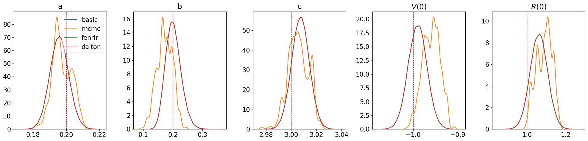
We compare the likelihood estimation for the four methods. Only Chrebtii MCMC algorithm differs from the rest because it uses MCMC to sample rather than the Laplace approximation.

plt.rcParams.update({'font.size': 15})
param_true = jnp.append(theta, x0)
var_names = ['a', 'b', 'c', r"$V(0)$", r"$R(0)$"]
fig, axs = plt.subplots(1, 5, figsize=(20,5))
for i in range(5):
    sns.kdeplot(basic_post[:, i], ax=axs[i], label='basic')
    sns.kdeplot(mcmc_post[:, i], ax=axs[i], label='mcmc')
    sns.kdeplot(fenrir_post[:, i], ax=axs[i], label='fenrir')
    sns.kdeplot(dalton_post[:, i], ax=axs[i], label='dalton')
    axs[i].axvline(x=param_true[i], linewidth=1, color='r', linestyle='dashed')
    axs[i].set_ylabel("")
    axs[i].set_title(var_names[i])
axs[0].legend(framealpha=0.5, loc='best')
fig.tight_layout()

Dalton Non-Gaussian Observations

Now suppose that the noisy observation model is

(1)\[\begin{equation} Y_{ij} \sim \operatorname{Poisson}(\exp{b_0 + b_1x_j(t_i)}), \end{equation}\]

where \(b_0 = 0.1\) and \(b_1 = 0.5\).

# simulate data
key = jax.random.PRNGKey(100)
b0 = 0.1
b1 = 0.5
Yt = jax.random.poisson(key,lam= jnp.exp(b0+b1*x))
obs_data = jnp.expand_dims(Yt, -1)

For non-Gaussian observations, please use daltonng. The inputs are the same as dalton with obs_weight and obs_var replaced by obs_loglik_i, which is the loglikelihood function of the observation. The rest of the process is the same as the Gaussian example.

def obs_loglik_i(obs_data_i, ode_data_i, ind, **params):
    """
    Likelihood function for the SEIRAH model in non-Gaussian DALTON format.

    Args:
        obs_data_i : Observations at index ``ind``.
        ode_data_i :  ODE solution at index ``ind``.
        ind : Index to determine the observation loglikelihood function.

    Returns:
        Loglikelihood of ``obs_data_i`` at index ``ind``.
    """
    b0 = 0.1
    b1 = 0.5
    return jnp.sum(jax.scipy.stats.poisson.logpmf(obs_data_i.flatten(), jnp.exp(b0+b1*ode_data_i[:, 0])))


def neglogpost_daltonng(upars):
    "Negative logposterior for non-Gaussian DALTON approximation."
    theta, X0, prior_pars = fitz_constrain_pars(upars, dt_sim)
    # non-Gaussian DALTON loglikelihood
    ll = rodeo.inference.daltonng(
        key=key,  # immaterial, since not used
        # ode specification
        ode_fun=fitz_fun,
        ode_weight=W,
        ode_init=X0,
        t_min=t_min,
        t_max=t_max,
        theta=theta,
        # solver
        n_steps=n_steps,
        interrogate=rodeo.interrogate.interrogate_kramer,
        prior_pars=prior_pars,
        # non-gaussian measurement model
        obs_data=obs_data,
        obs_times=obs_times,
        obs_loglik_i=obs_loglik_i
    )
    return -(ll + fitz_logprior(upars))

# optimization process
n_samples = 100000
upars_init = jnp.append(jnp.log(theta), x0)
upars_init = jnp.append(upars_init, jnp.ones(n_vars))
dalton_post = fitz_laplace(key, neglogpost_daltonng, n_samples, upars_init)

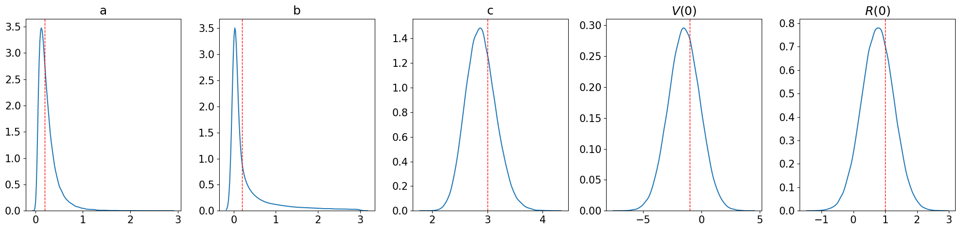
Results

fig, axs = plt.subplots(1, 5, figsize=(20,5))
for i in range(5):
    tmp_data = dalton_post[:, i]
    if i==0 or i==1:
        tmp_data = tmp_data[(tmp_data>0) & (tmp_data<3)]
    sns.kdeplot(tmp_data, ax=axs[i], label='dalton')
    axs[i].axvline(x=param_true[i], linewidth=1, color='r', linestyle='dashed')
    axs[i].set_ylabel("")
    axs[i].set_title(var_names[i])
fig.tight_layout()