Lorenz63: Chaotic ODE

In this notebook, we consider a multivariate ODE system called Lorenz63 given by

\[\begin{equation*} \begin{aligned} \frac{dx}{dt} &= \sigma(y - x), \\ \frac{dy}{dt} &= x(\rho - z) - y, \\ \frac{dz}{dt} &= xy - \beta z, \\ \xx_0 &= (-12,-5,28). \end{aligned} \end{equation*}\]

where \((\rho, \sigma, \beta) = (28, 10, 8/3)\).

import numpy as np
import matplotlib.pyplot as plt
import jax
import jax.numpy as jnp
from scipy.integrate import odeint

from rodeo import solve_mv
from rodeo.prior import ibm_init
from rodeo.interrogate import interrogate_kramer
from rodeo.inference.fenrir import solve_mv as fsolve
from rodeo.inference.dalton import solve_mv as dsolve
from rodeo.utils import first_order_pad
from jax import config
config.update("jax_enable_x64", True)

Suppose we observed data to help with solving the ODE and that they are simulated using the model

\[\begin{align*} \YY_i \sim \N(\xx(t_i), \phi^2 \Id_{2 \times 2}) \end{align*}\]

where \(t_i = i\) and \(i=0,1,\ldots 20\) and \(\phi^2 = 0.005\). We will first simulate some noisy data using an highly accurate ODE solver (odeint).

# ODE function
def lorenz0(X_t, t, theta):
    rho, sigma, beta = theta
    x, y, z = X_t
    dx = -sigma*x + sigma*y
    dy = rho*x - y -x*z
    dz = -beta*z + x*y
    return np.array([dx, dy, dz])

# it is assumed that the solution is sought on the interval [tmin, tmax]. 
tmin = 0.
tmax = 20.
theta = np.array([28, 10, 8/3])

# Initial x0 for odeint
ode0 = np.array([-12., -5., 38.])

# observations
n_obs = 20
obs_times = jnp.linspace(tmin, tmax, n_obs+1)
exact = odeint(lorenz0, ode0, obs_times, args=(theta,), rtol=1e-20)
gamma = np.sqrt(.005)
e_t = np.random.default_rng(0).normal(loc=0.0, scale=1, size=exact.shape)
obs = exact + gamma*e_t

We have a few different ways of solving this ODE. The first is using solve which do not use data at all. The other methods fenrir.solve_mv and dalton.solve_mv incorporate data to help the solution process. The setup for the three solvers are very similar:

# ODE function
def lorenz(X_t, t, theta):
    rho, sigma, beta = theta
    x, y, z = X_t[:,0]
    dx = -sigma*x + sigma*y
    dy = rho*x - y -x*z
    dz = -beta*z + x*y
    return jnp.array([[dx], [dy], [dz]])


# problem setup and intialization
n_deriv = 3  # Total state; q
n_vars = 3  # Total variables

# Time interval on which a solution is sought.
tmin = 0.
tmax = 20.
theta = jnp.array([28, 10, 8/3])

# The rest of the parameters can be tuned according to ODE
# For this problem, we will use
sigma = jnp.array([5e7]*n_vars)

# Initial W for jax block
W, lorenz_init_pad = first_order_pad(lorenz, n_deriv, n_vars)

# Initial x0 for jax block
x0 = lorenz_init_pad(jnp.array(ode0), 0, theta=theta)

# Get parameters needed to run the solver
n_res = 200
n_steps = n_obs*n_res
dt = (tmax-tmin)/n_steps  # step size
prior_pars = ibm_init(dt, n_deriv, sigma)

# prng key
key = jax.random.PRNGKey(0)

Next we define specifications required for dalton and fenrir. In particular, they expect observations to be of the form

\[\begin{equation*} \YY_i \sim \N(\DD_i \XX_i, \OOm_i). \end{equation*}\]

This translates to the following set of definitions for this 3-state ODE.

n_meas = 1  # number of measurements per variable in obs_data_i
obs_data = jnp.expand_dims(obs, -1) 
obs_weight = jnp.zeros((len(obs_data), n_vars, n_meas, n_deriv))
obs_weight = obs_weight.at[:, :, :, 0].set(1)
obs_var = jnp.zeros((len(obs_data), n_vars, n_meas, n_meas))
obs_var = obs_var.at[:, :, :, 0].set(gamma**2)

Now we can use the three solvers.

# rodeo
rsol, _ = solve_mv(key, lorenz, W, x0, tmin, tmax, n_steps,
                   interrogate_kramer,
                   prior_pars,
                   theta=theta)

# dalton
dsol, _ = dsolve(key, lorenz, W, x0, tmin, tmax, n_steps,
                 interrogate_kramer,
                 prior_pars,
                 obs_data, obs_times, obs_weight, obs_var,
                 theta=theta)

# fenrir
fsol, _ = fsolve(key, lorenz, W, x0, tmin, tmax, n_steps,
                 interrogate_kramer,
                 prior_pars,
                 obs_data, obs_times, obs_weight, obs_var,
                 theta=theta)

# exact solution
tseq_sim = np.linspace(tmin, tmax, n_steps+1)
exact = odeint(lorenz0, ode0, tseq_sim, args=(theta,), rtol=1e-20)

plt.rcParams.update({'font.size': 30})
fig, axs = plt.subplots(n_vars, figsize=(20, 10))
ylabel = [r'$x(t)$', r'$y(t)$', r'$z(t)$']

for i in range(n_vars):
    l0, = axs[i].plot(tseq_sim, rsol[:, i, 0], label="No Data", linewidth=3)
    l1, = axs[i].plot(tseq_sim, dsol[:, i, 0], label="DALTON", linewidth=3)
    l2, = axs[i].plot(tseq_sim, fsol[:, i, 0], label="Fenrir", linewidth=3)
    l3, = axs[i].plot(tseq_sim, exact[:, i], label='True', linewidth=2, color="black")
    l4 = axs[i].scatter(obs_times, obs[:, i], label='Obs', color='red', s=40, zorder=3)
    axs[i].set(ylabel=ylabel[i])
handles = [l0, l1, l2, l3, l4]
fig.subplots_adjust(bottom=0.1, wspace=0.33)

axs[2].legend(handles = handles , labels=['No Data', 'DALTON', 'Fenrir', 'True', 'obs'], loc='upper center', 
              bbox_to_anchor=(0.5, -0.2),fancybox=False, shadow=False, ncol=5)

<matplotlib.legend.Legend at 0x7b455ad8be20>

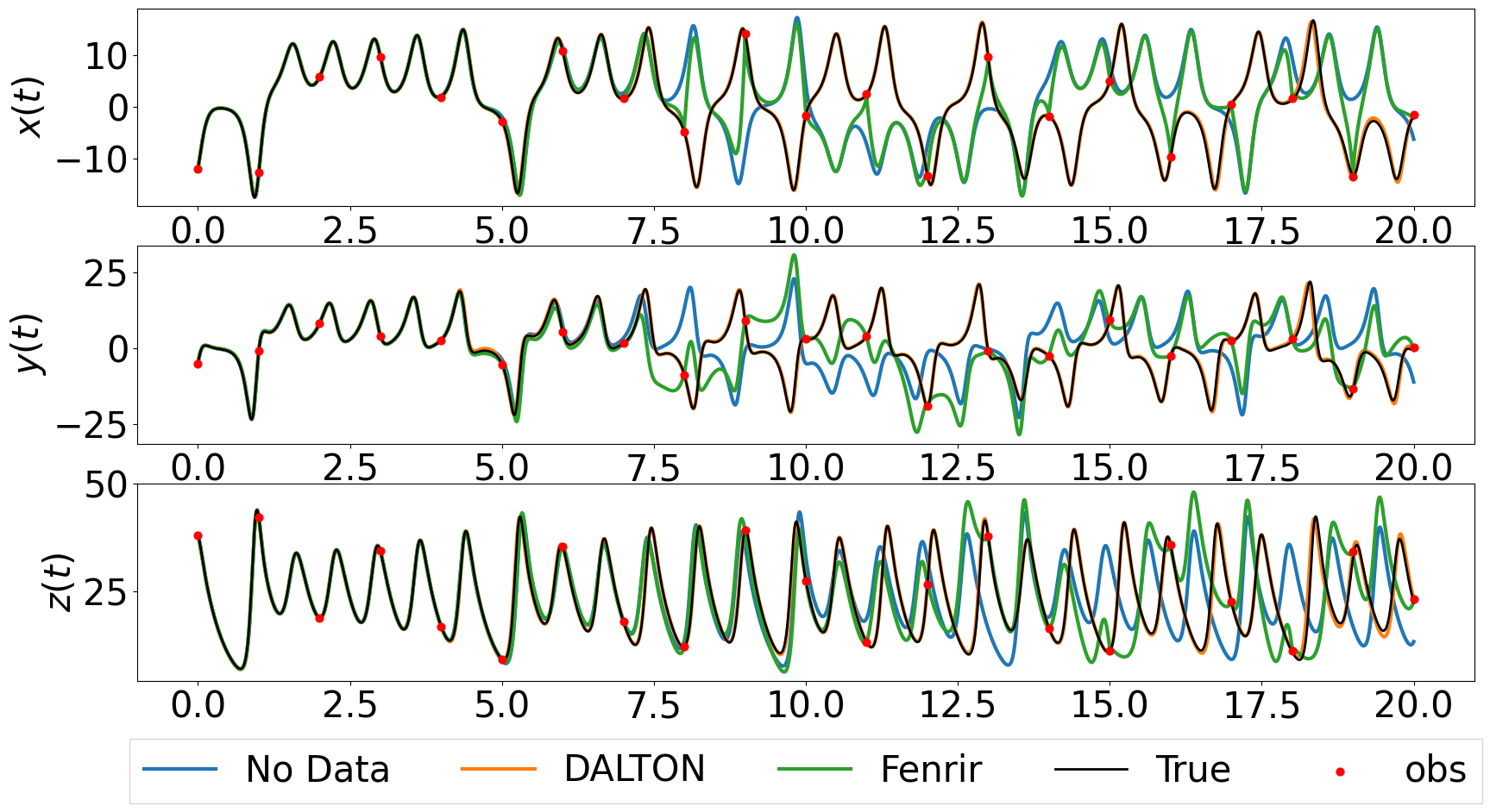
In the plot above, we see that only dalton is able to recover the true ODE solution beyond \(t>7.5\).